 Jacob Tomlinson
In Theo’s previous posts on storing high momentum data and its accompanying metadata we get some interesting insights into the future of cloud based data storage. In this post I’m going to cover how we are working with today’s NetCDF-based challenges, by making assumptions!

Every day we upload ~100K NetCDF files of varying sizes into AWS S3 which total around 7TB per day. We make these publicly available for research under the AWS Earth Open Data scheme. These files comprise four different datasets which are produced by four of our operational models (Global Atmospheric, UKV, MOGREPS-G and MOGREPS-UK). Each model has a number of variables such as air temperature, humidity and rainfall rate which can be thought of as sub-datasets.
Due to the nature of our weather/climate model (the Unified Model) and our Cray supercomputer every time a new time step is calculated by the model it is stored as a new file which begins its way through a post-processing pipeline to eventually end up as a NetCDF file in S3. This means there is a constant flow of new files being uploaded.
This data also goes out of date quickly: the forecast we produced last Monday for the weather last Thursday isn’t really going to have much value now. So we only hold seven days of data on S3. Old files are automatically purged by S3 Lifecycle Rules.
A common use case for this kind of data is in domain specific forecasting systems where the domain is affected by the weather. For example supermarkets are predicting what their customers will buy so they can ensure they have the correct stock, airlines are predicting precisely how much fuel they need to get from A to B to avoid carrying excess fuel and Local Authorities are predicting when road surfaces will become icy so they can deploy their gritters. Each of these systems take domain specific knowledge, historical knowledge and up to date weather forecasts to make their predictions.
These forecasting systems often ingest the files we produce one at a time, process them and update their own predictions. Therefore a good way to design a system to do this is to subscribe an AWS SQS queue to one of the AWS SNS topics that we make available through AWS Earth. Every time we create a new S3 file we send a notification to the topic which will be placed on your queue. These systems can then consume messages from the queue at its own leisure, download the object from S3 and process it.
This kind of system design works well for real time systems, but it isn’t great for academics and researchers who want to explore these datasets as a whole. It requires them to create queues, databases and ingest systems just to piece one of these datasets back together. Then they have to somehow load the thousands of files which make up the dataset and stitch them together into one coherent object. To avoid this problem we came up with Hypotheticubes!
Hypotheticubes
When we load a multidimensional array from a NetCDF file we refer to it as a cube, even if it doesn’t have three equal length dimensions. A cube is a high level representation of a data array and the metadata that describes it. When loading thousands of cubes which comprise a single high level dataset you can use a tool like Iris to combine them into a single representation of that high level object.
Sadly this can be slow and memory intensive. In order to create one high level object Iris must read the metadata from every single NetCDF file in order to work out how they fit together. Reading objects from an object store is a slow step compared to reading from local disk, because in systems like S3 you are trading latency for availability and parallelism.
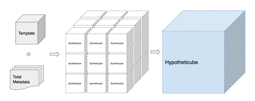
This brings us to our solution for loading a large number of NetCDF files: load one file and then using our knowledge of what the whole dataset should look like assume that the rest of the files exist. We can make these assumptions because we ran the model in the first place. We call this a hypotheticube.
Implementation
We have created an experimental implementation of hypotheticubes for our AWS Earth data which has resulted in three new open source Python libraries; iris-hypothetic, intake-hypothetic and mo-aws-earth. These libraries build on common open source libraries including Iris, pandas and intake. Let’s see what each one does.
Iris Hypothetic
In order to create our hypotheticube we need to create a representation of all the files which make it up, but we want to avoid loading each one individually. We do this by loading one cube and then cloning it as many time as we need whilst tweaking the metadata and data arrays as we go and then finally merging it together into one large cube.
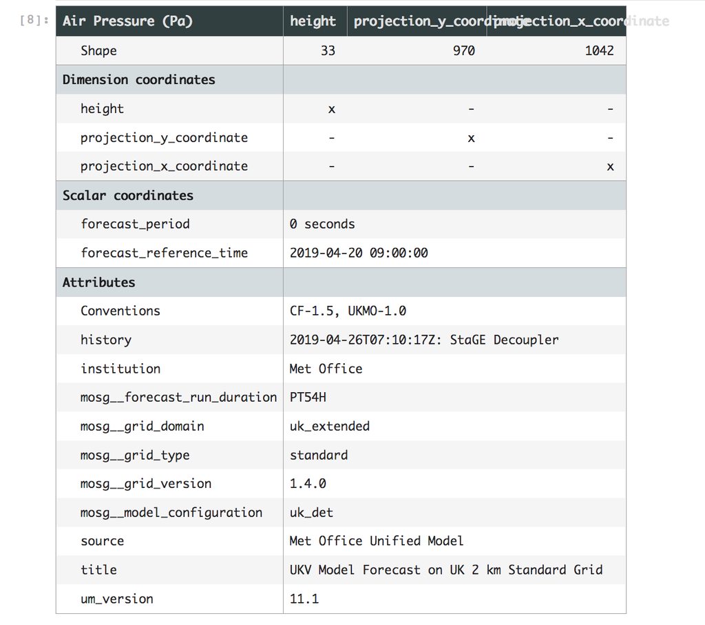
A cube is a set of metadata and a NumPy array-like object. When loading a NetCDF file with Iris it opens the file and reads the headers to get the cube metadata, it then creates a NetCDFDataProxy object which is a lazy representation of the array stored within the file. This object is lazy because it stores the path to the file and duck types as an array. No data is loaded into memory until someone tries to access the actual data values in the array. Only then will it load the data into an actual array object from the NetCDF file and then pass the array calls through to the true array object stored within.
In our hypotheticube implementation we need to do two things: avoid errors when files do not exist (our NetCDFDataProxy will throw an exception if the file doesn’t exist), and clone our initial cube replacing the metadata and NetCDFDataProxy object as many times as we need to.
To avoid errors when we hit missing data we have created a new version of the NetCDFDataProxy called CheckingNetCDFDataProxy. This implementation checks for the file’s existence before loading the array into memory and if the file doesn’t exist it creates a fully masked array of the same shape and size and returns that instead. This is important because we can’t be certain that all of the files in our dataset exist. Some files may still be working their way through the processing pipline and are not available on S3 yet. They could be uploaded to S3 but still replicating through S3’s eventual consistency model. Or even some models may have stalled part way through and only a subset of the data was actually generated. Those files hypothetically could exist, but don’t, so we need to mask them out if we can’t find them.
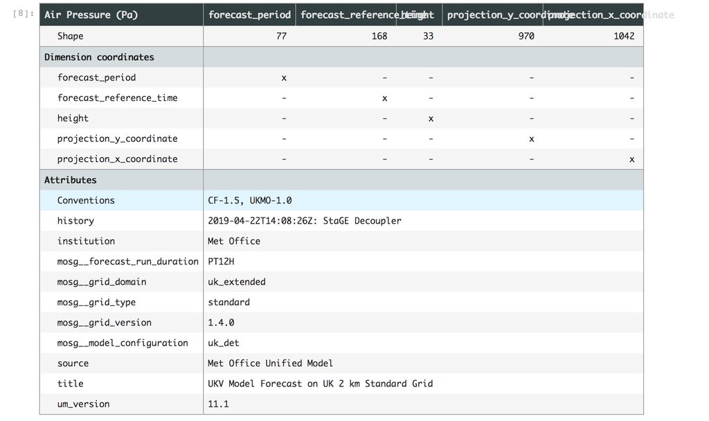
In order to create our hypotheticube we need an actual existing NetCDF file to start with. We call this the template cube. When calling iris-hypothetic we pass in our template cube along with a pandas dataframe of all the metadata combinations which could exist and a pandas series of where those files would be if they existed. We then iterate through the dataframe, create a copy of our template cube for each iteration, update the metadata and replace the NetCDFDataProxy with a new CheckingNetCDFDataProxy which points to the correct file. We refer to these constructed chunks as syntheticubes.
Once we have generated all of our syntheticubes we then use Iris’s built in functionality to merge and concatenate all of these into our final hypotheticube.
Intake Hypothetic
To create our hypotheticube with iris-hypothetic we needed three things; our template cube, our dataframe of metadata and our series of file paths. We can’t expect our users to know how to generate these, so we’ve created an intake driver to do this for them.
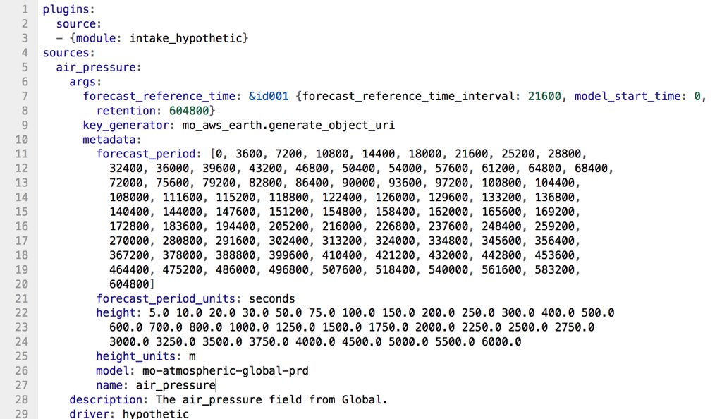
Intake is a data cataloging tool for Python which takes YAML catalog files that describe a dataset and run them through a driver which converts it into a useful data object such as a pandas dataframe or Iris cube. These catalogs and the complimentary data can then be shared easily with people.
The catalogs we’ve designed for iris-hypothetic contain information on all combinations of metadata that make up the dataset. There are three types of metadata which we capture in our catalog:
- Static metadata which doesn’t change between syntheticubes such as the units of the data.
- Iterative metadata such as the forecast period which is a list of dimension coordinates which are consistent across the dataset.
- Generative metadata which is a set of iterative metadata that needs to be calculated, such as the date of each day in the last week.
We take the product of the iterative metadata to construct our dataframe of all possible combinations of metadata. Once we have this we need to work out the file path for the file representing each set of metadata. To do this our catalog stores the Python import location of a function which will take a row of metadata and return the file path. We do this because our file paths could be something simple like /path/to/dir/{frt}_{fp}_{variable}.nc or in our case it is a hashed filename which can be reconstructed from the metadata. We use this function along with the metadata to construct the series of file paths.
Once we have our dataframe of metadata and series of file paths we need our template cube. To get this we begin hunting through our list of paths trying to load each one. We can’t guarantee they all exist so we just keep trying until we find one that loads, once one does we assume it is representative of all the other files and use it as our template. If we get all the way to the end of the list without finding a working template cube we raise an error.
Once we have these three objects we pass them to iris-hypothetic from within our intake driver and return the resulting hypotheticube.
MO AWS Earth
The last piece of the puzzle is to wrap everything up into one nice Python package.
The mo_aws_earth package contains a small amount of code (the function required for generating the file paths for the AWS Earth data), the YAML catalog files and all the dependencies required for the package. This means that anyone who wants to use the Met Office data from AWS earth can install everything they need in one line
conda install -c informaticslab mo_aws_earth
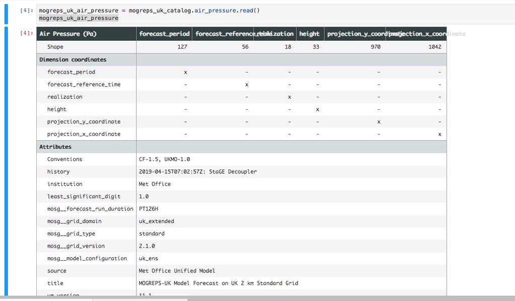
Then to use the data you can read any of the catalogs from intake by specifying the model and variable you want.
import intake
hypotheticube = intake.cat.mo_aws_earth.{model}.{variable}.read()
If you’re using this in IPython or a Jupyter Notebook you can tab complete the models and variables.
Exploring the data
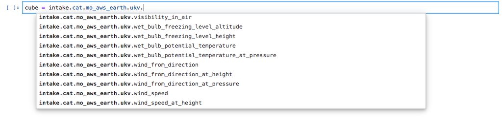
Now that we have our hypotheticubes we can begin exploring. Let’s load a hypotheticube of soil temperature from our UKV model.
Cube sizes
The first thing we might want to do is to check how big these hypothetical arrays are. We have a utility function within our jade_utils package called estimate_cube_size to estimate your in-memory size of a cube based on the shape and dtype.
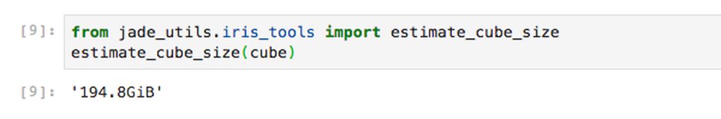
If we were to load our lazy array into memory it would take up 194.8GiB of RAM. If we want to do any science with it we need quite a lot of memory.
However, because we are using hypotheticubes based on Iris our data arrays are actually Dask arrays instead of NumPy arrays.
Dask allows you to work with arrays that are bigger than memory by streaming chunks of data from disk. It also allows you to distribute parallel calculations over many machines if you have a cluster available to you.
By using Dask it means that you can work with this ~200GB cube on your laptop, albeit slowly, or on a cluster running SLURM, PBS, Yarn or Kubernetes if you have access to one.
How hypothetical is our cube
To generate our hypotheticube we’ve made assumptions about what our dimensions look like. Continuing with our soil depth data from the UKV model we have assumed that we run the model every hour and we store the data for seven days. We then explored the metadata to find that the furthest into the future they simulated was five days. We then used these dimensions to construct our hypotheticube.
We can be certain about the model run frequency because we run the model and we can be certain about the storage time because we set the storage rules. However we cannot be certain of the model run length because we have assumed that all runs go out to five days.
To test this we can collapse all of our spacial dimensions with a mean to leave forecast reference time and forecast period and plot them. This will cause us to try to load every syntheticube of data and map out the dimensions we have made assumptions about.
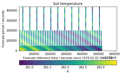
We can see in our plot that our assumption was mostly right. Some runs go to five days, some go out to 2.5 days, but the majority stop at one day. This is due to forecasts being expensive to run, and refining our prediction of the immediate future is more valuable than predicting further out.
We can also see that all of the recent forecasts (on the right hand side of the plot) are missing. This is due to the 24 hours delay which is added to the free AWS Earth data to distinguish it from our commercial offering.
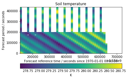
I had a closer look at the longer runs to see if there was any interesting finer detail. From this view the last run appears to only be part way through making it’s way to S3.
There are also a couple of missing chunks in the older runs. This could be for number of reasons but is most likely due to file corruption. If we had tried to load these chunks in the traditional way it would’ve failed to merge due non-contiguous data, but our hypotheticube masks them out and lets us continue.
From a glance we can see here that only around 25% of our hypothetical dataset really exists. However our assumptions were pretty good. Each orthogonal dimension is the right length to bound our dataset, it’s just that much of this dataset was never generated. If we had infinite time, money and computers we would run all of our models out to five days, and if we didn’t need to sell services to bring in revenue then we could release all of the data in real time. So despite our plots looking a little sparse we have correctly covered the hypothetical domain of our dataset.
We could update our catalogs to optimise this, perhaps by putting the long, medium and short runs into separate datasets with the correct forecast period dimensions. We could also update our catalog to start the forecast reference time 24 hours ago to avoid the right hand section which will always be blank. The downside to this workflow is that the only way to tell this is by working our way through the whole thing to see if anything is there. The upside is that we save lots of time in constructing our cube.
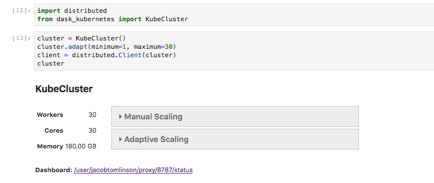
Distributing
One big benefit of having dask powered data arrays is being able to distribute our calculations. Calculating the mean above would have taken roughly two hours using a single core on my laptop, and that’s not including downloading the data. However I used dask-kubernetes on our Pangeo cluster to parallelise the operation, which took only four minutes.
Summary of assumptions
In order to create our hypotheticubes we’ve made a number of assumptions, let’s review them here:
- We know when we run our models and how they are configured.
- The majority of files will be made available on S3 eventually.
- The shape of a chunk is representative of every other chunk in the dataset.
- Chunks do not have unique unpredictable metadata.
- Constructing the same hypotheticube at a later date will be a different cube, relative to when it was loaded.
Knowing these assumptions allows us to decide whether they are acceptable to our work and whether we want to continue within this paradigm. But there are some issues which may prevent us from using this, such as reproducibility of science and provenance. The raw files still exist though so we can continue using them in a traditional way if these assumptions are not acceptable.
Conclusion
Working with hundreds of thousands of NetCDF files is a hard task. The frustrating thing is that all of the time and effort you need to put in to wrangle them isn’t solving your problem, it’s just busy work. By simplifying this step it allows more time to be devoted to the actual science of analysing and visualising the data in question. We hope that this demonstration of hypothetical datasets provides a fair trade off between being able to work with these datasets quickly and easily versus making some assumptions along the way.